Table of Contents
ToggleXGBoost or XGB stands for extreme gradient boosting. In XGB, feature importance points to how much a particular feature contributes to the model’s predictions. It is very important to know which features contribute most to the models’s prediction when we have a large number of columns in the dataset.
XGBoost provides several ways to compute and visualize the importance of features.
Feature Importance Using XGBClassifier or XGBRegressor
In XGBoost, we have built-in function to compute feature importance after fitting the model.
- Weight: It is the number of times a feature appears in a tree across all trees in the model
- Gain: The average contribution of a feature to the model. In simple terms, it means how much a feature improves the model’s performance.
- Cover: The average coverage of a feature which shows how frequently a feature is used to split the data.
Steps to get XGBoost Feature Importance :
Let’s predict the median house value using XGBRegressor for California districts using the fetch_california_housing dataset. Independent parameters are MedInc (Median income of the district) ,HouseAge (Median age of the houses in the district ), AveRooms (Average number of rooms per house in the district), AveOccup (Average number of occupants per household in the district), Lat (Latitude of the district), Long ( Longitude of the district ), Population (The population of the district), AveHouseAge: (Average house age in the district)
Train an XGBoost Model
import xgboost as xgb
from sklearn.datasets import fetch_california_housing
from sklearn.model_selection import train_test_split
import pandas as pd

data = fetch_california_housing()

X = data.data
y = data.target

# Convert X to a DataFrame with column names
X_df = pd.DataFrame(X, columns=data.feature_names)

# Convert y to a DataFrame (if you want to keep the target in a separate column)
y_df = pd.DataFrame(y, columns=["Target"])

# Now you can print X_df and y_df with column names
print("Features (X):")
print(X_df.head())


print("\nTarget (y):")
print(y_df.head())
Output
Features (X):
   MedInc  HouseAge  AveRooms  AveBedrms  Population  AveOccup  Latitude
0  8.3252      41.0  6.984127   1.023810       322.0  2.555556     37.88
1  8.3014      21.0  6.238137   0.971880      2401.0  2.109842     37.86
2  7.2574      52.0  8.288136   1.073446       496.0  2.802260     37.85
3  5.6431      52.0  5.817352   1.073059       558.0  2.547945     37.85
4  3.8462      52.0  6.281853   1.081081       565.0  2.181467     37.85

   Longitude
0    -122.23
1    -122.22
2    -122.24
3    -122.25
4    -122.25

Target (y):
   Target
0   4.526
1   3.585
2   3.521
3   3.413
4   3.422
Let’s now perform train test split.
# Train-test split
X_train, X_test, y_train, y_test = train_test_split(X_df, y_df, test_size=0.2, random_state=42)

# Train an XGBoost model
model = xgb.XGBRegressor(objective='reg:squarederror', n_estimators=100, random_state=42)
model.fit(X_train, y_train)
We get the fitted model with all its parameters
Get XGB Feature Importance
We can use model.get_booster().get_score() to get feature importance based on different metrics:
# Get feature importance
importance = model.get_booster().get_score(importance_type='weight')  # Options: 'weight', 'gain', 'cover'

We can change importance_type parameter with ‘gain’ or ‘cover’.

# Print the feature importance
print(importance)
Output
{'MedInc': 928.0, 'HouseAge': 560.0, 'AveRooms': 655.0, 'AveBedrms': 512.0, 'Population': 548.0, 'AveOccup': 744.0, 'Latitude': 884.0, 'Longitude': 833.0}
We can see a dictionary where keys are the feature names and values ae the importance score.
Visualizing Feature Importance
In the XGBoost library we have a built-in function called plot_importance() to visualize feature importance.
import matplotlib.pyplot as plt
# Plot the feature's importance
xgb.plot_importance(model, importance_type='weight', title="Feature Importance (Weight)", height=0.5)
plt.show()
Output
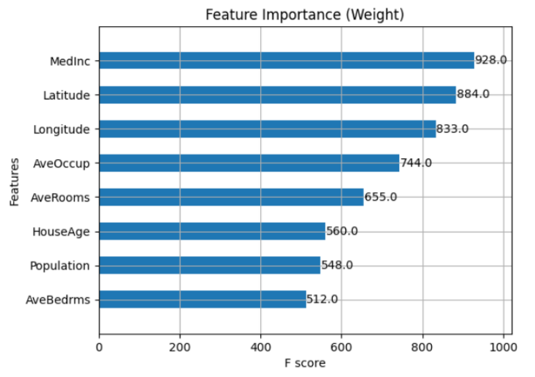
We can also change the importance_type to ‘weight’, ‘gain’, or ‘cover’ to visualize different metrics of feature importance.
Full code for XGBoost Feature Importance
Here’s a complete example using XGBRegressor with both Gain and Weight metrics:
import xgboost as xgb
from sklearn.datasets import fetch_california_housing
from sklearn.model_selection import train_test_split
import pandas as pd
import matplotlib.pyplot as plt

data = fetch_california_housing()

X = data.data
y = data.target

# Convert X to a DataFrame with column names
X_df = pd.DataFrame(X, columns=data.feature_names)

# Convert y to a DataFrame (if you want to keep the target in a separate column)
y_df = pd.DataFrame(y, columns=["Target"])

# Now you can print X_df and y_df with column names
print("Features (X):")
print(X_df.head())

print("\nTarget (y):")
print(y_df.head())

# Train-test split
X_train, X_test, y_train, y_test = train_test_split(X_df, y_df, test_size=0.2, random_state=42)

# Train an XGBoost model
model = xgb.XGBRegressor(objective='reg:squarederror', n_estimators=100, random_state=42)
model.fit(X_train, y_train)

# Get feature importance
importance = model.get_booster().get_score(importance_type='weight')  # Options: 'weight', 'gain', 'cover'

# Print the feature importance
print(importance)

# Plot the feature importance
xgb.plot_importance(model, importance_type='weight', title="Feature Importance (Weight)", height=0.5)
plt.show()
XGBoost Feature Importance Using sklearn's permutation_importance()
When we use XGBClassifier or XGBRegressor in a pipeline with sklearn, we can access and plot feature importance directly using sklearn’s permutation_importanc function.
from sklearn.inspection import permutation_importance

# Using permutation importance
result = permutation_importance(model, X_test, y_test, n_repeats=10, random_state=42)

# Plot permutation importance
plt.bar(range(X.shape[1]), result.importances_mean)
plt.xticks(range(X.shape[1]), data.feature_names, rotation=90)
plt.title('Permutation Feature Importance')
plt.show()
Output
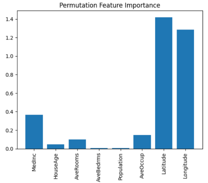
This method calculates feature importance by randomly permuting features and evaluating the decrease in the model’s performance.
XGBoost Feature Importance Using SHAP (SHapley Additive exPlanations)
SHAP values are another advanced method for calculating feature importance. It gives a unified measure of the impact of each feature on the model’s output. It gives us a deeper understanding of the relationships between features and predictions
Let’s explore the code of SHAP with XGBoost:
import shap

# Create a SHAP explainer object
explainer = shap.Explainer(model)

# Calculate SHAP values for the test set
shap_values = explainer(X_test)

# Plot the SHAP summary plot
shap.summary_plot(shap_values, X_test, feature_names=data.feature_names)
Output

We can see latitude, longitude and MedInc are majorly helping the model to predict.
Conclusion:
- XGBoost Built-in Methods: As discussed earlier, We can use get_booster().get_score() with parameters like weight, gain, and cover to get feature importance.
- Visualizing: We can use plot_importance() to easily visualize feature importance based on different criteria.
- Permutation Importance: Using sklearn’s permutation_importance provides an alternative, model-agnostic way to assess feature importance.
- SHAP: For a more detailed and interpretable measure of feature importance, SHAP values are a great option.
You can also read about other blogs on central limit theorem and how to implement early stopping in Tensorflow, Keras, and PyTorch